Of Working Faraday Cages and 5G

About a month ago, I ran across this funny tweet about people buying Faraday Cages or mental router covers to block 5G:

So apparently putting Faraday cages around routers has become a thing for the 5g conspiracy nuts and there are companies out there ready to cash in.

My sides are in orbit. pic.twitter.com/mGcud5Kb70

— 🦇Ansgar Odinson🦇 (@AnsgarTOdinson) December 2, 2020

I got really curious about what the Amazon reviews cumulatively looked like, so I did a small data collection of reviews from 33 different “Faraday cages” (and bags).

For folks who are unfamiliar with Faraday cages, these are encasings (typically of conductive mesh) which are used to block whatever is within the cage from electromagnetic fields. If put around a router, a Faraday cage would naturally block out all internet signal (and if it doesn’t, it wouldn’t actually be a Faraday cage). In other words, buying a Faraday cage to enclose your wireless router would defeat the purpose of having a wireless router.

Amazon Faraday Cages & Router Guards

Though attention to Faraday cages and router guards on Amazon appears to be pretty recent, some of these things have been sold on Amazon for several years. Pre-2020 reviews show that people initially bought these wanted to cover smart meters, which are often installed by electricity suppliers.

More recently however, people have been purchasing these covers to block from 5G Routers. In fact, there has been a notable increase in the number of verified reviews about these products.

View fullsize

Throughout the time span, verified reviews of the products range greatly from folks who are convinced that using a router guard has deceased their headaches/improved sleeping to people complaining that the product has made using the internet impossible. One common feature of the positive verified reviews was an emphasis on how the guards would block elites (electric companies and governments) from “getting inside my brain.”

However, there were also reviews of folks complaining that their internet was no longer accessible.

Another big reason why some of the Faraday cages/bags were poorly reviewed was that they were too small for routers. This was an especially common critique when people wanted to use cages for smart meters to cover their router.

Unverified reviews typically took on two types of flavors: (1) mocking those who had genuinely bought the product or (2) corrective information that tried to explain why these products are basically pointless. Notably, since the December 2, 2020 tweet, the number of unverified reviews has grown considerably.

Unsurprisingly, the most common positive sentiment words (when using the Bing sentiment dictionary) focused on its ease of use and how it “worked perfectly” (this was said both sarcastically and genuinely). Negative words either focused on the “harmful” effects of electromagnetic fields (headaches, cancer, etc.) or criticized the cages for being a scam or joke.

View fullsize

Though the results were pretty unsurprising, this was a good exercise in playing around with Amazon reviews! Plus, with my first semester of teaching over, I’m hoping I can be a more active blogger.

The data and code for this analysis can be found on my github, here.

Disney Plus Data and Chill ;)

On December 12, 2019, Disney unveiled its streaming service, Disney+, to the world. It received significant attention, both good and back, from the press—which makes sense, because over 10 million people signed up in the first day.

Twitter was also abuzz with conversations about Disney+ (see this string-of-tweet “news story” about Twitter activity on the first day). Several pointed out that shows, including new ones like The Mandalorian and oldies like Darkwing Duck, were trending soon after Disney+ was launched.

But what would activity look like after the first day?

To answer this question, I used Mike Kearney’s rtweet package to look at tweets posted from 11/14/19 to 11/18/19 that had one of the following keywords: disneyplus, disney plus, disney+, and disney +.

Timeline

As with any long-term (> 1 day) popular topic (like elections), tweets about Disney+ had a natural seasonality. People tweet less after midnight and pick back up at 6 or 7 a.m. the next day. While activity was still pretty high on the 14th, people tweeted less and less about it over time (as would be expected). There was a little over a million tweets in the corpus (n = 1,107,413).

View fullsize

Topic Modeling

I also ran an LDA topic modeling, which highlights the variety of conversations on Twitter about Disney +.

View fullsize

Noticeably, The Mandalorian, Hannah Montana, the Simpsons (which is on Disney+ in its original 4:3 format), and Bad Girls Club were talked about frequently enough to be (mostly) stand-alone topics. The Mandalorian hashtag (#themandalorian) was also a popular keyword in the corpus.

But we also see a variety of other topics, including one about the Nickelodeon and Netflix deal (which many people viewed as a response to Disney+’s explosive popularity) and another comparing Disney+ to other streaming services (like Netflix, Hulu, and HBO). In fact, Netflix was the third most frequent term in the dataset (behind Disney and Disneyplus).

(Some of the topics were obviously noisier than others. Topics with the little red “n” are “noisier” than the others, meaning that a large number of tweets with a high beta in that topic were not related to the topic labels. Many tweets in the “Bad Girls Club” topic, for example, don’t actually have to do with that show.)

Sentiment-Laden Words

I did a quick sentiment analysis as well, using the tidytext package (specifically, the bing sentiment lexicon). This allowed me to look at frequently used, sentiment-laden terms.

As with any sentiment analysis that is based on a lexicon, there are obvious limitations. The bing dictionary, for example, includes “trump” as a positive word, but it would count any mention of Donald “Trump” as well.

We can see a similar phenomenon here with the word “chill”, which Bing treats as a negative word. If you recall from the topic modeling results, “Disney+ and Chill” was a topic in-it-of-itself. In addition to using the specific phrase “Disney+ & Chill” (which is a snowclone from “Netflix & Chill”), we see people trying to come up with their own variants, including “Disney+ and Thrust” and “Disney+ and Bust”.

For a quick and dirty analysis, this was a pretty fun corpus of tweets to go through! You can check out my code at my Github.

The Grammar of "A Thing": Using R to Study Digital Corpora

One of the things I love most about my field (Communication) is its unique passion for building corpora. While there is an obvious value to studying a large, well-studied, pre-structured corpora like LOB or COCA (e.g., multiple scholars working on one dataset increases knowledge about that dataset, reproducibility, etc.), some research questions require more specialized text data.

This is often the situation that I find myself in. If I want to study a linguistic phenomenon in a specific register—like the use of “a thing” in English tweets—I usually have to build my own corpus. So how does one do that?

I’ll break my process down into four broad steps: (1) armchair linguistic-ing, (2) creating the corpus, (3) finding your linguistic phenomenon, (4) corpus analysis.

01. Armchair Linguistic-ing

I became primarily interested in this construction because of its frequency in language use. In spoken English, sentences like, “oh yeah, that’s a thing” are commonplace, even in formal-ish settings, like classrooms (I’m in a J-School, so it’s not unusual to hear someone say, “Yeah, AP style is a thing”).

I’ve always liked this construction, because “a” and “thing” are particularly vague English words. The determiner “a” (as in “I gave her a book”) is indefinite, meaning it refers to something non-specific (contrast this to “I gave her the book”). And “thing” is so broad, it could refer to any tangible, inanimate object. A watch, a book, a stroller, a ticket to Disney—all of these things are things. But when we put “a thing” together, it can suddenly take on a whole new meaning. When someone says, “AP style is a thing”, they mean “people know about AP style” or “AP style is popular”. In this context, the “a thing” is more than an indefinite determiner and a vague noun. Rather, it signifies some degree of importance.

But is this always the case? I wasn’t sure. So, I turned to my corpus building skills to find out.

I figured there could be four general places that “a thing” could be situated in. The first is the subject, like in the sentences below:

1. A thing needs to be done.

2. A thing just arrived.

The second possibility is in the object position, such as in the examples below:

1. I know a thing or two about school.

2. I made a thing.

It is also possible that “a thing” is used as a predicate noun/nominative. It is also a subject complement, because it completes a linking verb (in English, “to be”). This is the structure I was most interested in.

1. This is a thing.

2. That has been a thing for a long time.

And finally, we’ll look into object complements, such as in the examples below:

1. He considered the party a thing.

2. He cooked his friends a thing.

Now that I knew what I was looking for, it was time to build and parse my corpus.

02. Building Your Corpus

The first thing you’ll need to think about is where you want to get the data from. Do you want to look at journal articles? Fiction novels? Text messages between friends?

I settled on Twitter for a few reasons, the most important of which was “it is an informal register that is easy to get.” I figured the feature I was looking for would likely not be in a formal register, like news stories or presidential speeches. However, Twitter (and social media language as a whole) is simultaneously beautiful and frustrating in its kind-of-formal, kind-of-informal language norms (beautiful in that language evolves so quickly, frustrating in that there are way too many people who use prescriptivism to put down other people’s tweets).

If you are trying to access the Twitter RestAPI through R, I strongly advocate using rtweet, by Mike Kearney. It’s a really cool package, and a great way to build interesting Twitter corpora at your leisure.

library(rtweet)
#?search_tweets
rstats_tweets <- search_tweets(q = '"a thing"',
                               n = 1000000, 
                               retryonratelimit = TRUE) #max 18,000 every 15 minutes

head(rstats_tweets, n = 5) #looks at the top 2 tweets

This search yielded about 500,000 tweets (510,574, to be exact). To identify whether the bigram “a thing” would be used as a subject, object, predicate, or object complement, I would need to annotate this bad boy.

Right now, I’m using the R clearNLP package, with back ends to spaCy and CoreNLP. I tend to use the latter more (coreNLP) because I’ve gotten better results. But spaCy is much faster and has additional support. I strongly encourage it for those who are both R and Python-proficient (it can also support word vectors and has a great displaCy visualizer).

library(rJava)
library(tokenizers)
library(cleanNLP)

In order to use cleanNLP, you’ll need to interface with the back end (either coreNLP or spaCy).

#cnlp_init_tokenizers() #initializes tokenizer backend
cnlp_download_corenlp()
cnlp_init_corenlp("en", anno_level = 2)
# cnlp_init_spacy

Once you have done this, you are ready to parse your corpus! For the purposes of this exercise, I’m going to use some toy data (parsing the full corpus took about 2 days—I had about 20 million dependencies total).

Toy Data

If you notice, 8 of the 9 sentences are the ones in my previous examples.

toy_data <- data.frame(id = c("s1", "s2", "o1", "o2", "sp1", "sp2", "sp3", "dc1", "dc2"),
                       sentence = c("A thing needs to be done.", "A thing just arrived.", 
                                    "I know a thing or two about school.",
                                    "I made a thing.", 
                                    "This is a thing.", 
                                    "Is summer camp a thing?",
                                    "That has been a thing for so long.", 
                                    "He considered the party a thing.", 
                                    "He made his friends a thing."))

starttime <- Sys.time()
full_corpus_dep <- toy_data$sentence %>% as.character() %>%
  cnlp_annotate(as_strings = TRUE, doc_ids = toy_data$id) %>%
  cnlp_get_dependency(get_token = TRUE)
endtime <- Sys.time()

You want to make sure that you indicate the doc_ids of the data, as that is what you will use to re-align the dependency information to the original tweet or sentence.

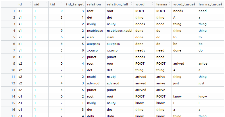
Once you do this, you should get a data frame that looks something like this:

Let’s break what cnlp_get_dependency produces. Each row represents one dependency relationship. Each column represents some information about that dependency (e.g., what document or sentence the dependency is in, what words the dependency relationship is linking, etc.)

A brief interlude to help us understand dependency grammar… Dependency grammar interprets two words as having a dependency (relationship) between them. This differs from constituency grammar, which breaks down word relationship into phrases, not dependencies. An important skillset in this work is being able to read the results of one and interpret it as the other (e.g., see dependency relations and conceptualize them as phrases, or see phrases and construct the dependencies).

Because dependencies focus on relationship between two words, we can conceive of a dependency relationship as having a “word”, a “wordtarget”, and a “relation”. Consider the very simple example of “I run.” In this sentence, we have a subject and a verb. In dependency grammar, the verb is the “root” or the center of the sentence. Therefore, each of your sentences will usually have a root. Arrows lead out from the root to other words (these are the “word targets”). Thus, if “run” is the root verb, then the word target “I” is the subject to that verb.

Let’s now look at each column in more detail. The <id> is pretty obvious: it’s the document id, or <doc_ids>, you indicated previously. The <sid> is the sentence number. For most tweets and sentences, the <sid> number will be a 1. However, blog posts, news articles, products reviews, and other longer documents are all likely to have multiple sentences. The <tid> refers to the token number of the word. There is also a <tid_target>, which is the token number of the word target.

The six other columns are: <relation>, <relation_full>, <word>, <lemma>, <word_target>, and <lemma_target>. The <lemma> and <lemma_target> are the lemmatized forms of the word and word_target (for example, the words “thinking”, “thought”, and “thinks” can be represented by the lemma /think/. Using the lemmatized form meant I largely did not have to worry about tense issues.

The <relation>, <word>, and <word_target> are the meat of the dependency analysis. The first “dependency” of a sentence is usually the ROOT verb. Let’s return to our “I run.” Example below.

As you can see, the “run” verb is identified as the root. This is not really a dependency, but more an identification of what the root verb is (hence why there is no actual <word>, and why the <tid> is 0). The second row identifies a <nsubj> dependency “relation”, with the root verb “run” as the <word>, and the noun subject “I” as the <word_target>.

There are many (many) possible dependency relations. You can find a list of them here.

There is some older documentation that can also be potentially useful here (this version of the dependencies is no longer maintained).

Let’s now apply this knowledge to our toy data.

03. Finding your Linguistic Phenomenon

Recall that our goal is to identify whether the bigram “a thing” appears as a subject, object, predicate, or object complement.

Let’s do so by identifying all the dependencies for which “thing” is a <word> or <word_target> (the “a” in “a thing” will be identified as a determiner <word_target> to the “thing”).

thing_word <- subset(full_corpus_dep, word == "thing")
thing_target <- subset(full_corpus_dep, word_target == "thing")

Notice that the “a thing” dependency shows up in the <thing_word> subsetted data. But the more useful dataset for us is the <thing_target> data.

Notice that, if in the subject position, the “thing” <word_target> has a <nsubj> (noun subject) <relation> to a verb. In the object position, the “thing” <word_target> has a <dobj> (direct object) <relation>. In the predicate position, the “thing” <word_target> is the ROOT (if you check the <word> data, you will also note a <cop>, or copula, <relation> from the verb “to be” to the “thing” <word>). In the object complement position, the “thing” <word_target> has an <xcomp>, or an “open clausal complement” <relation>.

Below is an image of all the dependency relationships I was interested in, as related to the “a thing” bigram.

View fullsize

Side note: While the toy data plays nicely, real data isn’t always perfectly parsed. For example, I had about 2,000 tweets where a copula-predicate relationship was identified as a subject-verb(“to be”)-object relationship (these had a “nsubj” + “det” + “dobj” relationship, but the root lemma was “be”—this meant they were initially coded as “objects” but, upon further examination, I subset them to the predicate list).

04. Corpus Analysis

Now that we know what the relationships are, we can re-aggregate to the tweet level. My corpus had a few instances (<10) where “a thing” was used twice. In all these instances, however, the “a thing” bigrams were in the same position.

subject <- subset(thing_target, relation == "nsubj", select=id) %>% mutate(subject = 1)
object <- subset(thing_target, relation == "dobj", select=id) %>% mutate(object = 1)
predicate <- subset(thing_target, relation == "root", select=id) %>% mutate(predicate = 1)
complement <- subset(thing_target, relation == "xcomp", select=id)  %>% mutate(complement = 1)

toy_data2 <- merge(toy_data, subject, by = "id", all.x = T) %>% 
  merge(object, by = "id", all.x = T) %>%
  merge(predicate, by = "id", all.x = T) %>%
  merge(complement, by = "id", all.x = T)
toy_data2[is.na(toy_data2)] <- 0

Let us now turn to the results of the full data.

Results

As we can see, the bigram “a thing” is most likely to appear in the object position (“I made a thing”) or predicate position (“This is a thing“).Rarely is “a thing” used in the subject position (e.g., “Love the phrase ‘a meteoric rise’, a thing a meteor has never done”). Fewer than 250 tweets had “a thing” in the object complement position.

“A thing” in the Predicate position

As I expected, tweets that used “a thing” in the predicate noun position discussed a subject as popular, socially important, or at least well-known. These tweets usually followed a similar structure: the word “thing” is the root. The word_target “a” is a determiner to “thing”, and the lemma “to be” (representing “is”, “are”, “was”, and “were”) is a copula to “thing”. Finally, the “nsubj” relationship would link the noun word_target to the “thing” word (this is why we need the thing_word subsetted data).

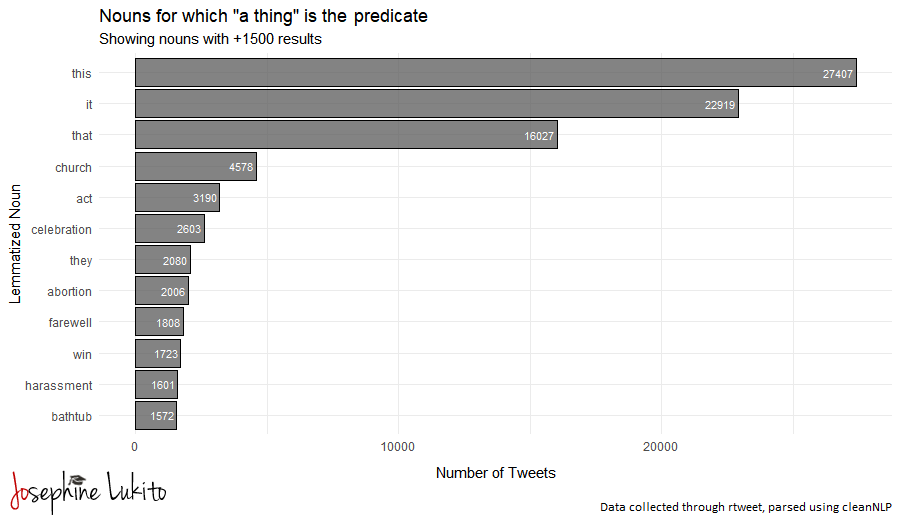
So what are nouns are described as “a thing”?

The figure above shows that, when "a thing" is a predicate, it often link to demonstrative determiners (this, that) or the pronoun "it". We also see some more specific nouns, such as ‘church”, “abortion”, and “harassment”.

Many of these tweets were exclamations (e.g., “I didn’t know this was a thing!” or “OMG this is a thing?!” or “Had no idea this was a thing!!”). Some were questions, about whether something was “still a thing”: “I grew up being told about thick and thin. Is that still a thing[?]”

“Church” appeared often in tweets like, “Is church still a thing?” and “How is church and religion still a thing?” In at least one instance, a tweet was incorrectly parsed: “separation of church and state is a thing, you know that right little @mike_pense?” (the parser coded this as ([NP] separation ([PP]of ([N] church)) ([CONJ] and) ([N] state), rather than treating “church and state” as a conjunction within the preposition phrase).

Many people also described abortions as a thing (or not a thing). A few tweets noted “Abortions are a thing” to note the frequency with which they occur. One tweet said “Late term abortions should not be a thing”, focusing on a specific type of abortions. Another said, “Post-term abortion is not a thing”, referring specifically to President Trump’s coinage.

“A thing” in the object position

Let us now turn to the use of “a thing” in the object position. In these cases, “a thing” is still relatively vague. If you “make a thing”, you’re not necessarily saying the thing you made is popular or well-known—you may simply be happy that you did it (e.g., “I did a thing!”).We can explore this structure more by looking at the verbs associated with the “a thing” bigram in the object position. The dependency relationship would be a dobj from the word_target “a thing” to a verb.

The figure below displays the verbs that appeared at least 5000+ tweets, for which “a thing” was a direct object.

Keep in mind that these verbs are lemmatized (therefore the lemma “know” represents “know” and “knew”). By far, the most common verbs used were “to do” and “to make” (as in “I did a thing” and “I made a thing”). This is followed by “to have”, “to know”, “to miss”, and “to learn”.

For example, one tweet said “I made a thing for Pokemon fans and Kingdom Hearts fans [Image]”. Note that the author provided additional info (a prepositional phrase and an image) to describe the “thing”. Another user tweeted, “It looks bad but i did a thing [image].” Many of these tweets expressed some pride over doing, making, creating, having, buying, or owning “a thing”. This was almost always accompanied by pictures of what the “thing” was.

Some tweets also referenced love, as in “love don’t mean a thing” or “love don’t cost a thing”. About 6000 tweets used the verb “change”, and were often about commenting on other people’s worth (e.g., “don’t change a thing!”)

Overall, I really enjoyed doing this analysis. It’s been more difficult to do this analysis with my Ph.D work picking up, but I’m glad I can still find the time every now and again.

Attending the R Forwards Women's Package Workshop (Hosted by R-Ladies Chicago)

This weekend, I had the pleasure of attending an R Forwards Women's Package Workshop. It was hosted and run by members of R-Ladies Chicago: Angela Li and Stephanie Kirmer.

Though I have attended and run many one or two hour workshops, this was my first long-day, single-topic workshop (9:30 to 4:00 pm) and I thoroughly enjoyed the experience! It’s definitely a format that would be useful to teach more complex topics, like software development and package building. There was a lot of info-in-brain-cramming, but I also felt like I learned a ton in a very short time span.

Attendees of the 2019 R Forward Package Workshop, taught by Angela and Stephanie of R Ladies Chicago!

The session was broken down into a couple broad topics: package development, git+r, unit testing, documentation, and package sharing (e.g., licences, indicating dependencies, CRAN). This made the material useful for both specific-use packages (e.g., building a data wrangling package for my specific research group) and for more public-facing packages (e.g., a package that one would want to upload to CRAN).

Top 5 Things I Learned:

1. The usethis package is so convenient and important for package development. For example, the function

   usethis::create_package("~/Desktop/mypackage")

   will create the skeleton of the package files for you, including folders for R-code, the “man” folder (“man” stands for manual), and description/namespace files. This makes package building so much earlier! You can learn more about it in Wickham’s R package book.

2. Using the “::” operator allows you to see the exported variables or functions in a package namespace. But if you really want to see under the hood “:::” allows you to see everything (there’s some more about it on StackOverflow), including the functions that are not publicly exported.

3. Semantic Versioning - How have I only learned about this now, despite attending several data carpentry workshops and classes?! I am such a stickler for version recording, even in my non-computational work (I have been subconsciously semantic versioning my human content analysis codebooks), and it’s so nice to finally have a specific phrase associated with this process.

4. A quote from my favorite slide of the day: “If the first line of your #rstats script is

   setwd("C:\Users\jenny\path\that\only\I\have")

   I will come into your lab and SET YOUR COMPUTER ON FIRE 🔥.”

   Confession time: I do this a lot! 🙈 ::embarrassed:: In terms of workflow, I am generally quite sloppy about separating projects and keeping relative paths. I first read about projects in R for Data Science, but I never took the lesson to heart until this weekend. I know… it’s bad given how much I code. So I guess I’ll be “konmari-ing” my R code this semester(i.e., create an Rproject space for each of my projects)!

5. A great tip from Stephanie’s top tweet (about Git): “when you screw up a git merge, you can use git reset --hard master@{"300 minutes ago"} with any time quantity you want in there to get back to where things were a period of time ago.“

.@data_stephanie shares her most popular tweet of all time and mind = blown 🤯 #RLadies #RForwardsChi pic.twitter.com/nCh97AE28j

— R-Ladies Chicago (@RLadiesChicago) February 23, 2019

Extra Bonus: Differencing vs. Logging Time Series Data

I happened to also sit next to economist Dweepobotee Brahma, which was a great coincidence since I’ve been binging time series models and papers for the past year. I happened to randomly gripe about how economic data is often processed (i.e., logged). She was kind enough to explain to me why economists did this, and why growth rates are so important to the research in economics and econometrics. Having been taught by a political scientist, whose questions are not as focused on exponential relationships, I didn’t know much about this alternative treatment/perspective on time series data, and it was really interesting!

I’m starting to wonder if this is especially important to modeling follower growth. Nearly all follower count time series I’ve analyzed have been fully integrated I(1), if not to I(2). Often I will first- or second- difference this as a way to make the series stationary. However, I’m realizing a logarithmic transformation is probably more appropriate for what we try to measure (implicitly, it’s a growth rate question).

Conclusion

Overall, I’m really, really glad that I was able to attend this workshop. It’s definitely up there on my “favorite R workshops ever” list. Organizationally, there were a lot of little things I wanted to take back to my workshop strategy (for example, this was the first workshop I attended where we used post it’s to indicate whether we needed help with specific tasks) and obviously it was great for advancing my R skills.

One of the most important “big picture” lessons I learned was that if I want to actually do software development in R (or any programming language), I have to be more organized about my code. I am organized when it comes to data management, but am definitely less-so with my scripts and functions. Workflow wise, I want to get on top of this by the end of the semester.

I’m also one step closer to completing a major R-new-year’s-resolution: Build an R package! I have a couple of functions that I rely on for data wrangling operationalized text data to time series data, so I’m eager to wrap them all up in a neat little package for future use.

And finally, attending the workshop was a great reminder about how amazing the R community is, both offline and online. That’s one of my favorite parts about being an R programmer—the community makes it easy to be excited about learning R.

I am so grateful to Angela and Stephanie for hosting this amazing workshop, and to R Forwards for sponsoring my attendance. If you are interested in checking out the materials from this weekend, they have made the workshop material available here.